Neural-Network Fractals

Last weekend, on a whim, I asked GPT-4 “Please teach me how to create simple neural networks in Python using PyTorch.” I wasn’t sure how well that would go, but figured it was worth a try.

I not only learned how to do that, but found out that GPT-4, at least when it isn’t making things up, is an amazing tutor. It not only provided the relevant code, but explained how it works, helped walk me through some snags installing the required libraries, and is continuing to explain how to tweak the code to implement new features of PyTorch for more efficient network training. I can now analyze arbitrary .csv file data with neural networks. Amazing.

I had heard that, given sufficient data, a complex enough network, and enough training time, neural networks can learn the patterns underlying almost anything. So I decided to see how well it would do with the task I always start out with when learning a new language — generating images of the Mandelbrot Set.

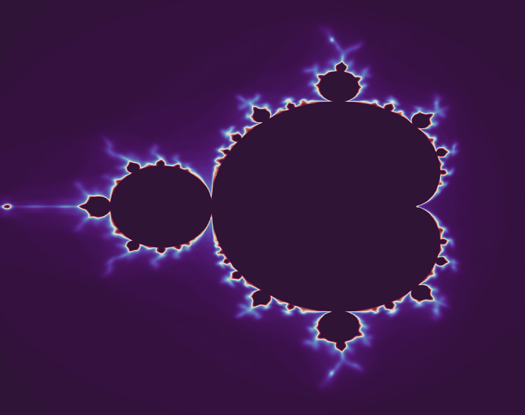
An image of the Mandelbrot Set, as imagined by a 1500-neuron network.

That’s far from the best image of the Mandelbrot Set I’ve ever created — but there’s a reason. As JFK said, we do such things “not because they are easy, but because they are hard.” The Mandelbrot Set is, after all, a literally infinitely-complex object. Keep zooming in, and there will always be more somewhat-similar-but-not-quite-identical detail.

Creating such images is traditionally done by calculating the number of iterations for each point in the image, and coloring the point accordingly. The neural-network approach I used (which to be clear is not even approximately the most efficient way to do it) does it somewhat differently. Data on millions of randomly-chosen points and their associated iteration levels is stored in a .csv file. This file is then read into memory and used as the training (and verification) dataset to train a feedforward neural network to learn what iteration levels are associated with what points. Then, when training is done, this network is used as the function to draw the Set — it is queried for each point in the image instead of doing the iteration calculations for that point.

This network doesn’t have vision. It is given a pair of numbers (representing the location in the complex plane) and outputs a single number (its guess at the iteration level). The image is somewhat unclear because it was, in effect, drawn by an “artist” who cannot see. It learned, through massively-repeated trials, what the Set looks like. Nobody “told” it, for example, that the Set is symmetrical about the X axis. It is, but the network had to figure that out for itself.

At first, the images only approximately resembled the Mandelbrot Set. But neural network design is still very much an art as well as a science (at least for now), so increasing the width and depth and switching to Kaiming initialization (to avoid the vanishing gradient problem) resulted in an image that meets my initial goal: the locations of the second-level Mandelbrot lakes are visible. The coloration at the edges even hints at the infinitely-thin “Devil’s Polymer” links that connect the mini-lakes to the main lobes.

GPT-4 still does get some things wrong. When asking it to guide me through tasks like obtaining a diamond pickaxe and then an Elytra in Minecraft (tasks that I know well), it mostly did a good job, but didn’t seem to know, for example, that hunger, Endermen, and Pillagers are not things that you have to be concerned about when playing on Peaceful mode. But even so, I was able to follow its directions to accomplish those goals.

This is a new form of intelligence, if perhaps not sentience just yet. I’ve often said that I love living in the future. It just got dramatically more futuristic.

Posted in Algorithms, Coding, Fractals, Machine Learning / Neural Networks, Minecraft, Python | Tagged , , , , , | Leave a comment

The Old XOR Switcheroo

Suppose you have two binary integers A and B.

You want to swap them so that A becomes B and B becomes A, but you don’t have any extra memory. If you start with A=B , for instance, the information that was in A is lost.

Can this be done? Surprisingly, yes, using the XOR swap algorithm:

A = A XOR B;
B = B XOR A;
A = A XOR B;

A is first changed to be a bitwise XOR of itself and B. As long as B is still available, the information in A could be recovered by repeating the operation.

Next, B is XORed with the new value of A. This leaves B with the information that was originally in A. Since A still contains the combination, both pieces of information are still recoverable.

Finally, A is XORed with B. Since B contains the original value that was in A, A will now contain the other half of the information — the value originally in B.

Now, for the story behind the story…

The idea, once known, is easy enough to prove — but I wanted to know who had come up with it. I tried asking ChatGPT, and it knew exactly the algorithm I was talking about, and rephrased what it does. It then very confidently said that it was discovered by Richard Hamming in the 1950s, and gave textbook and paper citations of his to back it up.

Very impressive — except it seems to be a hallucination. Maybe Hamming did discover the XOR swap. It wouldn’t surprise me at all. (After all, he’s the Hamming in “Hamming codes.” But the two references ChatGPT gave were duds. Hamming does mention XOR in his book on communications, but only briefly, where it is relevant to error-correcting codes.

Posted in Algorithms, Assembly, Coding, Digital, Math | Tagged , , , | Leave a comment

Kilofarad

I know what kilo means. I know what farad means. But even so, I never thought I’d have a use for the word kilofarad — let alone have one on my desk.

One kilofarad (two 500F caps in parallel). Hard to believe, but there it is.

The farad, named after Michael Faraday, is the SI unit of capacitance. It is equal to one coulomb of charge per volt. One coulomb is equivalent to one amp-second: one amp of current flowing for one second transfers one coulomb of charge.

This suggests an experiment: Charge a parallel pair of 500F capacitors (a kilofarad compound capacitor) at a constant 1A, as measured by a trusted DVM. Put another meter in DC voltage mode across the capacitor, and log the rate of change of voltage. (One kilofarad should be one millivolt per coulomb of charge, so we can use voltage as a “gas gauge” for how much charge is stored.)

For a textbook 1kF capacitor charged at a constant 1.0 amps, voltage should rise at 1mV per second, or 3.6V per hour. Since the power supply will have to provide some overvoltage in order to make up for any system losses and keep 1A flowing, this experiment has to be carefully monitored to avoid overcharging the capacitors.

It’s not that they’re particularly expensive. It’s that a 1kF capacitor, charged to 2.7V, stores some 3.6kJ of energy. That’s enough to lift even my 100kg posterior some 3.33m, or almost 11 feet, straight up. To imagine what a failed cap would be like, imagine sitting on an ejection chair powered by an explosive charge powerful enough to launch a large adult ten feet in the air. That’s how much energy is in there — at only 2.7V!
(“Danger: Low Voltage”…??)

Charging at a constant 1A (kept generally within 1mA) resulted in the following voltage/charge curve. (Upon reaching 2.75V, the power supply was disconnected and the capacitors allowed to self-discharge. Effective capacitance was not measured past that point.) Interestingly, voltage rose more slowly with increasing charge. The orange curve on the chart shows effective capacitance to each point. When charged to at least 1.1V or so, the two 500F capacitors do seem to make a one-kilofarad pair.

…At least, if there has been no significant loss of charge. Measuring that will need either a controlled-current load, or simultaneous monitoring of both voltage and current, since any simple resistive load will likely experience significant changes in resistance as it heats up.

Voltage (blue, volts) and effective capacitance (orange, kilofarads)
Posted in Analog, Components, Electronics, Fundamentals, Mad Science, Reviews, Science, Toys | Tagged , , , , , , , , , , , , , | Leave a comment

Mini Museum: TRS-80 Model 200

A Tandy 200 — essentially, a Model 100 with 2x the display area and a clamshell case.

The “Tandy 200” (Tandy had by then dropped the TRS-80 label) is an upgraded TRS-80 Model 100. The most noticeable upgrade, of course, is the new clamshell display, with twice the display area as on the Model 100. Better cursor keys are another improvement.

The -200 also has banked memory. Presumably for backwards compatibility, the system memory is limited to 32kB, but the -200 can access three (?) memory banks of 32kB each, by switching between them. Kind of like having three different computers in one, I guess?

The processor in the Model 100, -102, and Tandy 200 is an Intel 8085. Despite the similarity in number to the Intel 8088 powering the original IBM PC, the 8085 is essentially an 8080 with a few tweaks and a single-rail 5V power supply to make integration easier. It has more in common with Z80 machines like the Timex/Sinclair 1000 than it does with x86 machines.

While the Tandy 200 is an improvement over the Model 100, it turned out to not be as popular. Even the Model 102 — really just an updated 100 — sold more units. The reasons given were price (the larger display no doubt cost more) and size. While the -200 is significantly thicker and heavier than a Model 100, the laptops of just a few years later would make it almost look like a pocket computer. (IBM PC Convertible with optional printer module, we’re looking at you.)

While I don’t have nearly as much personal history with this one as with my Model 100 (which was my main computer for a few years until I built the ‘486), it’s interesting to see the differences.

I should put an ESP32 on the RS232 port as a dongle and let it browse the Web via lynx…

Posted in BASIC, Drexel, Mini Museum, Nostalgia, Tools | Leave a comment