The Short Way Around

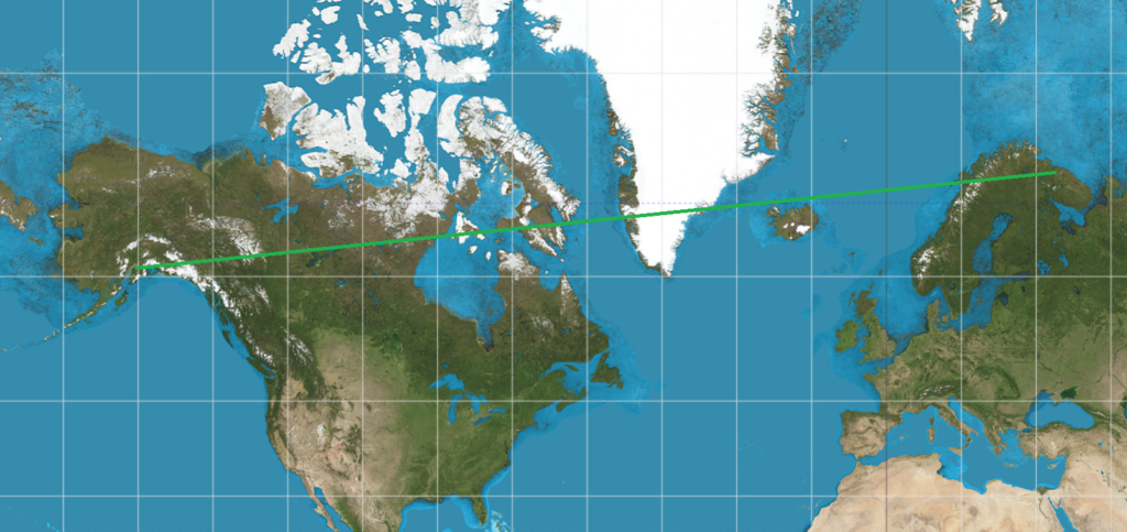
Although we’re all familiar with the flat Mercator map of the Earth, it exaggerates areas at high latitudes. More importantly for navigation, it also suggests very inefficient routing — routes calculated by taking the starting and ending latitude and longitude and using linear interpolation to find intermediate waypoints works well enough for low latitudes, but could end up suggesting a route that’s more than 50% longer, at high latitudes.

Consider a hypothetical flight from Murmansk (ULMM) to Anchorage (PANC). Although both cities are between 60 and 70 degrees north latitude, the shortest path between the two passes almost directly over the pole. In contrast, drawing a straight line between the two on a Mercator projection would imply a best path across Scandinavia, passing north of Iceland, then over Greenland and most of Canada before approaching Anchorage from the East.

It looks convincing, but the Flat Earth path will take a lot longer…
The Great Circle route. Seen on a globe, this is the obvious shortest path.

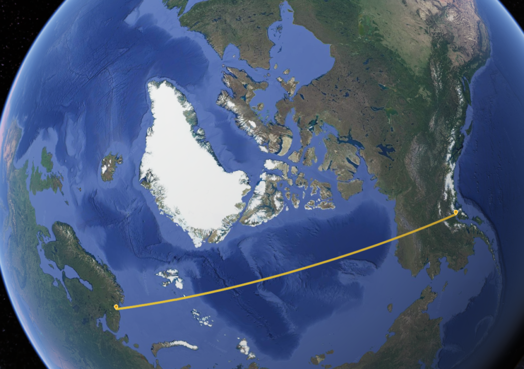
So Great Circle routes are faster — but how can you calculate them? It seems complicated — but a key observation can help. The Great Circle route is the shortest route between two points along the Earth’s surface because it is the projection of the actual shortest path through space.

With this insight, we have a plan of attack:

  • Consider the Earth to be a unit sphere. This is slightly inaccurate, but it works well enough.
  • Convert the starting and ending points to XYZ Cartesian coordinates;
  • Choose how many points to interpolate along the route;
  • Interpolate these linearly (directly through XYZ-space — through the body of the Earth);
  • Extend the distance from the origin of each point so it sits on the unit sphere
    (I.E. compute the distance of the 3D point from the Earth’s core, and extend it to 1.0 length);
  • Compute the latitude of each point as arcsin(z), and the longitude as arg(x+yi).

While this method doesn’t split the path into equal length segments, it gets most of them fairly close, with segment distances varying by 20% or so. If desired, this could be adjusted by changing the points selected along the initial linear path.

Posted in Algorithms, Aviation, Coding, Math | Tagged , , , , , | Leave a comment

For Loop Gotchas

Be careful when writing loops with unsigned variables. The compiler’s idea of an end condition might not match yours.

When working on a program to produce fractal laser-engraver art, I stumbled across a strange problem. I could call a function to draw a fractal at levels 0 through 6, all of which worked fine, whether individually or called in a for loop.

When I went to draw them in reverse order, however, the program crashed — and it didn’t make sense as to why. The code in question was something like:

dim as ulongint x
for x=6 to 0 step -1
drawObject(x)
next x

This worked fine forwards (for x=0 to 6) but crashed somewhere around level 2 when run in reverse — even though all levels worked great individually.

I eventually figured out that the bug was due to the variable in the for loop. Instead of iterating from 6 down to zero and then stopping, for loops (in FreeBasic as well as C) blindly decrement the variable and then check the end condition.

So, in C, a line which reads

for(uint8_t x=6;x>=0;x--){doTheThing(x);}

will never return. It will get down to zero, decrement and wrap back to all-ones. Since this is a value greater than zero, it will continue.

In the case of the fractal image, I had unknowingly asked it to compute an 18.4667-quintillion-level Koch curve. This figure would have four-to-the-18.4667-quintillionth-power segments.

No wonder it crashed!

Posted in BASIC, C, Coding, Fractals | Leave a comment

Moore’s Law

If you’re living inside an explosion, you may not notice it, if it’s something you’ve been used to. Our Universe continues to not only expand, but (as we found out only about twenty years ago), it’s accelerating. Still, life seems to go on much as it always has — nothing much seems noticeable at our timescale.

Even when things do change appreciably in our lifetimes, sometimes the change is so gradual that you almost don’t notice. Over the years, personal computing devices’ storage has grown from bytes to kilobytes in the 1970s, through megabytes and gigabytes into the terabyte realm today, with petabytes on the horizon for consumer devices.

What’s hard to grasp intuitively is that each of those multiplier name changes represents a thousandfold increase. (Or, a 1024-fold, if you’re a computer engineer and not a marketer.) So, compared to the earliest PCs, modern devices can store literally billions of times more information. Large server farms from the 1970s could be stored in one directory of a modern PC. We’re experiencing a technological explosion.

Even since 2004, changes are dramatic. Here’s a “then-and-now” shot of two USB Flash drives. The larger, silver one is a 128MB drive from 2004; the smaller one (that’s basically the size of the USB-A port plus a token plastic grip) is a 512GB drive from 2021.

…Less is more?

That’s roughly four thousand times larger — and it’s a fraction of the physical size.

I think I’ll mount it to a vacuum tube for ergonomics.

Posted in Current Events, Digital Citizenship, Nostalgia, Uncategorized | Tagged , , , , | Leave a comment

Wireless Sketch Updates for ESP8266

With the onboard WiFi capability that the ESP8266 and ESP32 boards provide, the natural next question is, can they be reprogrammed this way, too?

As it turns out, they can — and it’s fairly straightforward, thanks to the ArduinoOTA library (OTA standing for Over-The-Air.) Once programmed with an initial sketch to get the OTA functionality up and running (as well as provide the SSID and password for your WiFi), ESP8266 (and ESP32) boards can accept new sketches via their WiFi connection. There is even provision in the stock Arduino IDE to do this.

Random Nerd Tutorials has an excellent tutorial (as I guess you’d expect) on how to get started with this. If you’re in a hurry, here are my impressions after playing with it for an evening or so:

  • (The tutorial says Python 2.7 is required. I had it already, so I can’t say for sure.)
  • Add the Arduino core for your ESP8266 board (NodeMCU etc.) if you haven’t already.
  • Open the “Files–>Examples–>Ardruino OTA–>Basic OTA” example sketch. (If you can’t find it, the code is available here.
  • Modify the SSID and password lines to match your local WiFi network setup.
  • Compile and upload your sketch, using a USB cord like a cave dweller this one last time.
  • Since you’re connected via USB, you have Serial Monitor available, so you can watch it connect to the network (unless you’re like me and entered the wrong network name at first.)
  • Once it’s up and running, you should see a “Network Ports” section under Ports in the Arduino IDE. If all went well, you should see your board here. Select it and you can now upload to it this way.

That’s it — except for a few details that might not come to mind right away:

  • Make sure your new sketch also has the same OTA functionality (and your SSID and password) baked in, or once it is successfully uploaded, your board will no longer be listening for OTA updates, until you sheepishly ask the museum to borrow your USB cable back.
  • I’ve had the best luck with putting the ArduinoOTA.handle() call at the end of loop(). I suspect it might tend to use up most (or all) of the processor’s time, otherwise.
  • Don’t be a hog with time in your loop — do what you need and pass control back to the OTA handler.
  • If you move your board to a new network with a different SSID and/or password, it will need to be updated before the move. Unless you write the sketch to handle multiple networks, this will disconnect it from the former network.

This kind of functionality suggests some interesting applications — like encasing a system completely in resin, to be programmed wirelessly and powered by light or magnetic couplings.

Posted in Arduino, C, Digital, HOW-TO, Internet, Networking | Tagged , , , , , , , , | Leave a comment